Introduction
Basic use of the trip package.
Data input and validation
Tracking data is in essence a grouped series of one-dimensional data1 records.
It is grouped because we may track more than one object, each with its on independent time sequence.
It is one-dimensional because the topology of the data is a linear stream of values. It makes sense that time is constantly increasing, and it is the primary dimension of the process. (Location is often something that we must estimate, but time is usually directly measured and robust).
Commonly we have records in a data frame, and the primary workflow is to provide the trip() function with information about the spatial locations, the temporal data, and the grouping.
The data may contain any other columns, and in general they can be called anything and be in any order, but the simplest way to create a trip is to put the first four columns as X, Y, date-time, grouping.
## Warning in assume_if_longlat(out): input looks like longitude/latitude data,
## assuming +proj=longlat +datum=WGS84summary(tr)
##
## Object of class trip
##   tripID ("id") No.Records   startTime ("tms")     endTime ("tms") tripDuration
## 1             1          5 2020-10-27 23:24:45 2020-10-27 23:24:49       4 secs
## 2             2          5 2020-10-27 23:24:50 2020-10-27 23:24:54       4 secs
##   tripDistance meanSpeed maxSpeed
## 1     566.1822  509563.9 531029.7
## 2     690.8841  621795.7 987347.3
##
## Total trip duration: 8 seconds (0 hours, 8 seconds)
##
## Derived from Spatial data:
##
## Object of class SpatialPointsDataFrame
## Coordinates:
##         min       max
## x  1.000000 10.000000
## y -1.573627  1.243202
## Is projected: FALSE
## proj4string : [+proj=longlat +datum=WGS84]
## Number of points: 10
## Data attributes:
##       tms                      id
##  Min.   :2020-10-27 23:24:45   1:5
##  1st Qu.:2020-10-27 23:24:48   2:5
##  Median :2020-10-27 23:24:50
##  Mean   :2020-10-27 23:24:50
##  3rd Qu.:2020-10-27 23:24:52
##  Max.   :2020-10-27 23:24:54
(There may be only one group, but we have to be explicit, with a column that identifies at least one group).
When a print or summary is made the data are presented in terms of their grouping, with some handy summary values. When converting to sf or sp form as lines these summary values are recorded with each “multi”-line.
Simple plotting
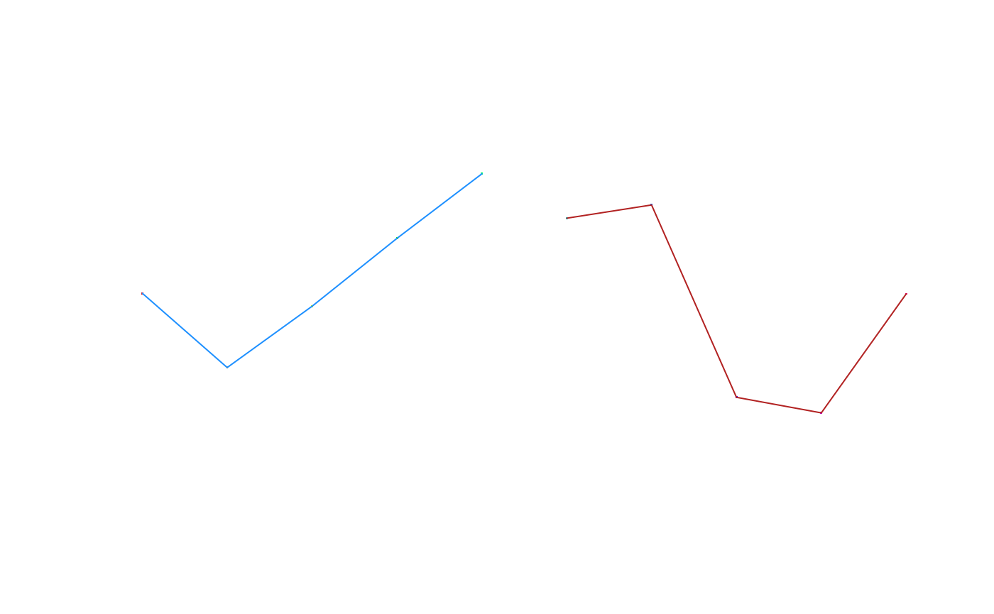
To plot a trip we use base graphics in the usual ways.

The trip object acts as a sp data frame of points, but with the underlying grouping as lines when that is relevant.
Gridding for time spent
There is a key functionality to determine the time spent in area on a grid, by leveraging the rasterize() generic function in the raster package. Any raster object may be used, so the specification of pixel area, extent and map projection is up to the user. (The trip line segments must all fall within the raster).
tg <- rasterize(tr)
plot(tg, col = c("transparent", heat.colors(25)))
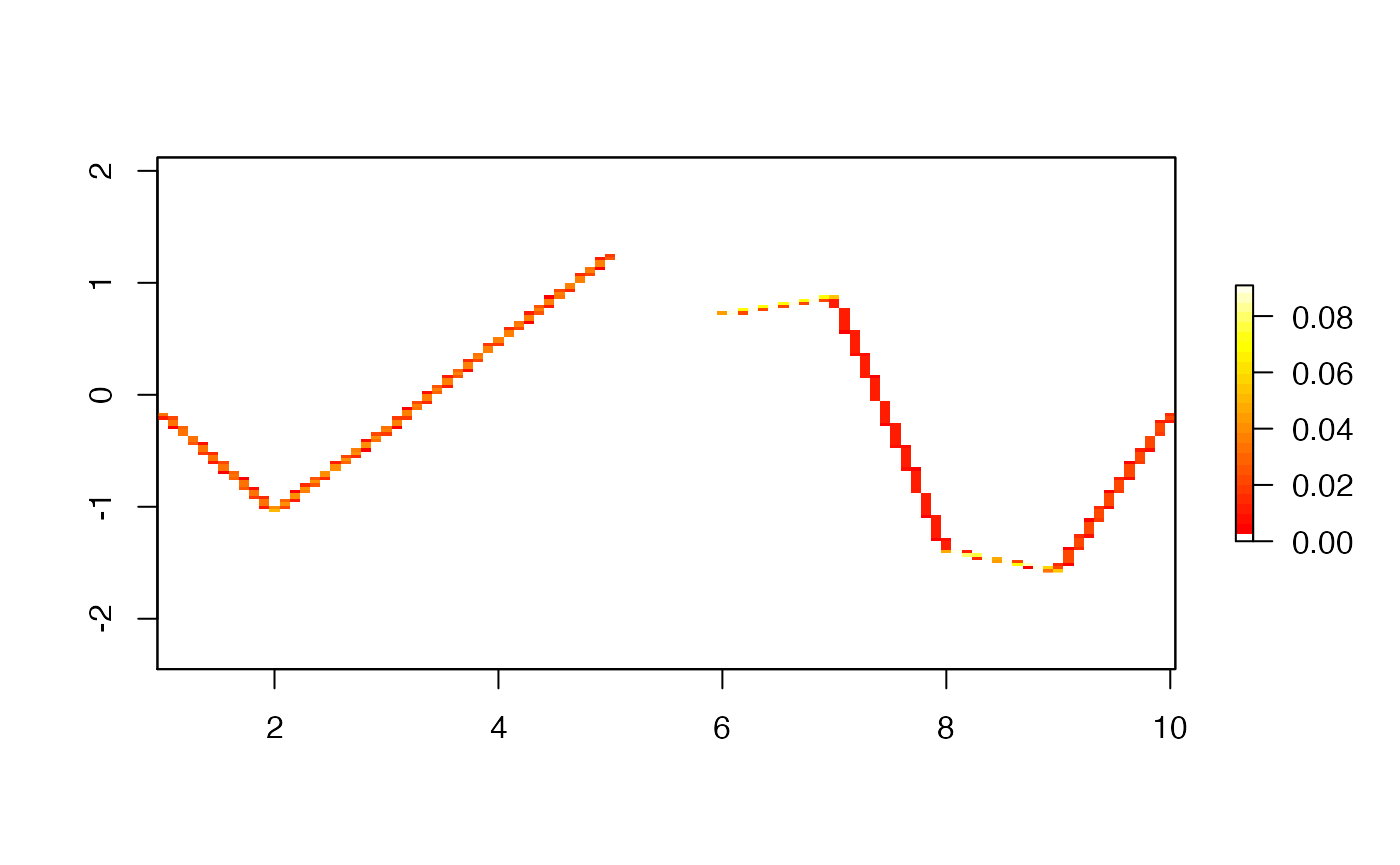
As with raster::rasterize() the field used may be chosen, by default the time difference between each point in a trip is used, and the final grid contains the sum of these durations.
There is an older version of this in the tripGrid.interp function that uses approximate methods by allowing interpolation to an ‘equal time’ step.
Reading from Argos files
Service Argos has provide various message formats, and the readArgos() function understands some variants of the ‘PRV’ form. Multiple files can be provided, and all messages will be normalized and turned into a trip object with no need for the user to group or clean them in any way.
argosfile <-
 system.file("extdata/argos/98feb.dat", package = "trip", mustWork = TRUE)
argos <- readArgos(argosfile)
##
## Longitudes contain values greater than 180,
##
##
##
##
## Data fully validated: returning object of class tripsummary(argos)
##
## Object of class trip
##    tripID ("ptt") No.Records   startTime ("gmt")     endTime ("gmt")
## 1            2163        134 1998-02-01 03:32:32 1998-02-24 07:33:35
## 2            6072        150 1998-02-01 03:30:03 1998-02-28 23:16:54
## 3            6073        149 1998-02-03 20:47:38 1998-02-28 23:11:56
## 4            6074        194 1998-02-01 01:51:52 1998-02-28 09:27:23
## 5            6075        160 1998-02-01 17:25:23 1998-02-28 23:17:54
## 6            6076        157 1998-02-01 03:26:28 1998-02-24 07:34:53
## 7            9301        203 1998-02-01 03:33:42 1998-02-28 06:07:30
## 8            9302         87 1998-02-01 05:09:25 1998-02-26 16:10:40
## 9            9303         12 1998-02-01 01:07:29 1998-02-06 09:12:07
## 10           9373        207 1998-02-01 01:51:09 1998-02-24 07:36:01
## 11           9374        191 1998-02-02 15:34:44 1998-02-28 21:36:10
## 12           9375        109 1998-02-01 01:50:39 1998-02-27 03:48:20
## 13           9376        136 1998-02-01 17:26:47 1998-02-22 16:59:45
## 14           9377        115 1998-02-02 07:17:31 1998-02-22 23:48:03
##     tripDuration tripDistance  meanSpeed     maxSpeed
## 1   23.1674 days    1865.7487   6.441413    38.003719
## 2   27.8242 days    1894.6721   6.128032   145.251489
## 3  25.10021 days    1825.6069   6.004080   178.192971
## 4  27.31633 days    2241.5163  12.318890   577.145877
## 5   27.2448 days    1730.3140 114.630616 17393.145193
## 6  23.17251 days    2277.5287   8.759922   158.324144
## 7  27.10681 days    3107.6614  42.621290  6649.062042
## 8   25.4592 days    1034.6549   3.079610    24.671973
## 9  5.336551 days     160.2035   2.563500     7.675708
## 10 23.23949 days    2370.2940 165.640436 32335.751235
## 11   26.251 days    1863.8627  89.308060 15503.634403
## 12 26.08172 days    2531.4993  14.742137   502.168226
## 13 20.98123 days    1521.9433   5.339746    47.063667
## 14 20.68787 days    1164.6709   4.730864    49.179020
##
## Total trip duration: 28422949 seconds (7895 hours, 949 seconds)
##
## Derived from Spatial data:
##
## Object of class SpatialPointsDataFrame
## Coordinates:
##               min     max
## longitude 318.281 328.453
## latitude  -54.689 -51.449
## Is projected: FALSE
## proj4string : [+proj=longlat +datum=WGS84]
## Number of points: 2004
## Data attributes:
##     prognum         ptt           nlines          nsensor      satname  class
##  Min.   :920   Min.   :2163   Min.   : 2.000   Min.   : 1.00   D:1001   Z:  0
##  1st Qu.:920   1st Qu.:6074   1st Qu.: 3.000   1st Qu.:32.00   J:1003   B:403
##  Median :920   Median :9301   Median : 4.000   Median :32.00            A:376
##  Mean   :920   Mean   :7547   Mean   : 4.428   Mean   :29.93            0:704
##  3rd Qu.:920   3rd Qu.:9374   3rd Qu.: 5.000   3rd Qu.:32.00            1:420
##  Max.   :920   Max.   :9377   Max.   :58.000   Max.   :32.00            2: 83
##                                                                         3: 18
##      date               time              altitude   transfreq
##  Length:2004        Length:2004        Min.   :0   Min.   :401648599
##  Class :character   Class :character   1st Qu.:0   1st Qu.:401649265
##  Mode  :character   Mode  :character   Median :0   Median :401649474
##                                        Mean   :0   Mean   :401649505
##                                        3rd Qu.:0   3rd Qu.:401649747
##                                        Max.   :0   Max.   :401650517
##
##       gmt
##  Min.   :1998-02-01 01:07:29
##  1st Qu.:1998-02-07 16:19:52
##  Median :1998-02-13 04:40:36
##  Mean   :1998-02-13 20:18:48
##  3rd Qu.:1998-02-20 07:48:41
##  Max.   :1998-02-28 23:17:54
##
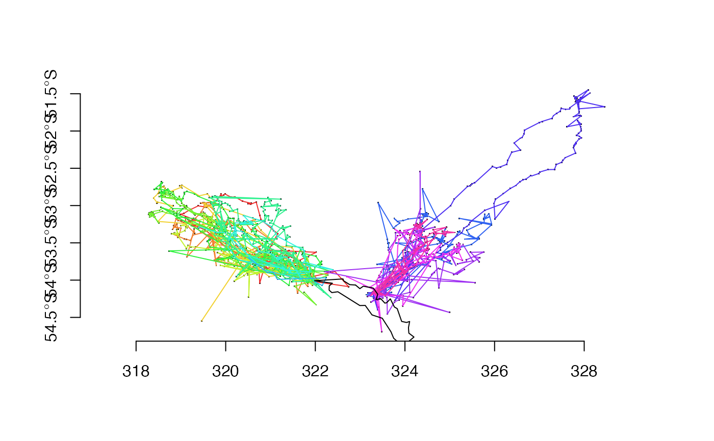
Note that the form of the coordinates is native to the PRV file, and in this case contains longitude values that are greater than 180. Some forms of these files provide wrapped forms, but in general the data are read as-is.
(We need “world2” because we are at 40W, but +360).
Destructive filtering
There are some classic data filters based on speed and angle, and we may chain these together for some cheap improvements to track data, or use them separately.
argos$spd <- speedfilter(argos, max.speed = 4)  ## km/h
mean(argos$spd)  ## more than 5% are too fast
## [1] 0.748503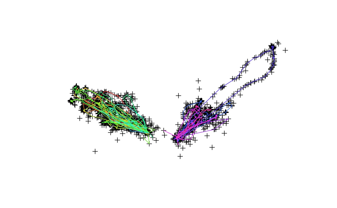
argos$sda <- sda(argos, smax = 12)  ## defaults based on argosfilter, Freitas et al. (2008)
mean(argos$sda)
## [1] 0.8687625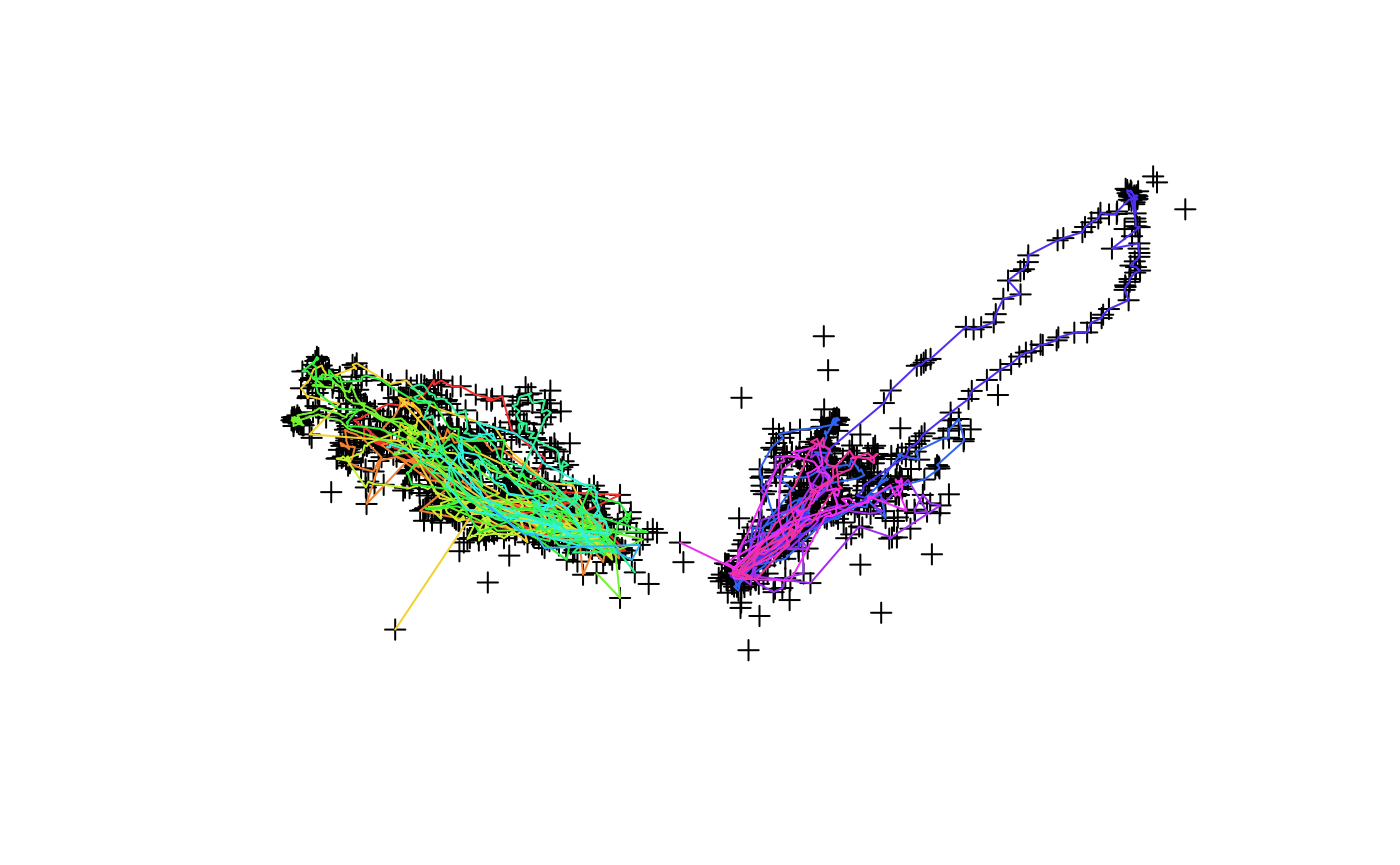
Map projections
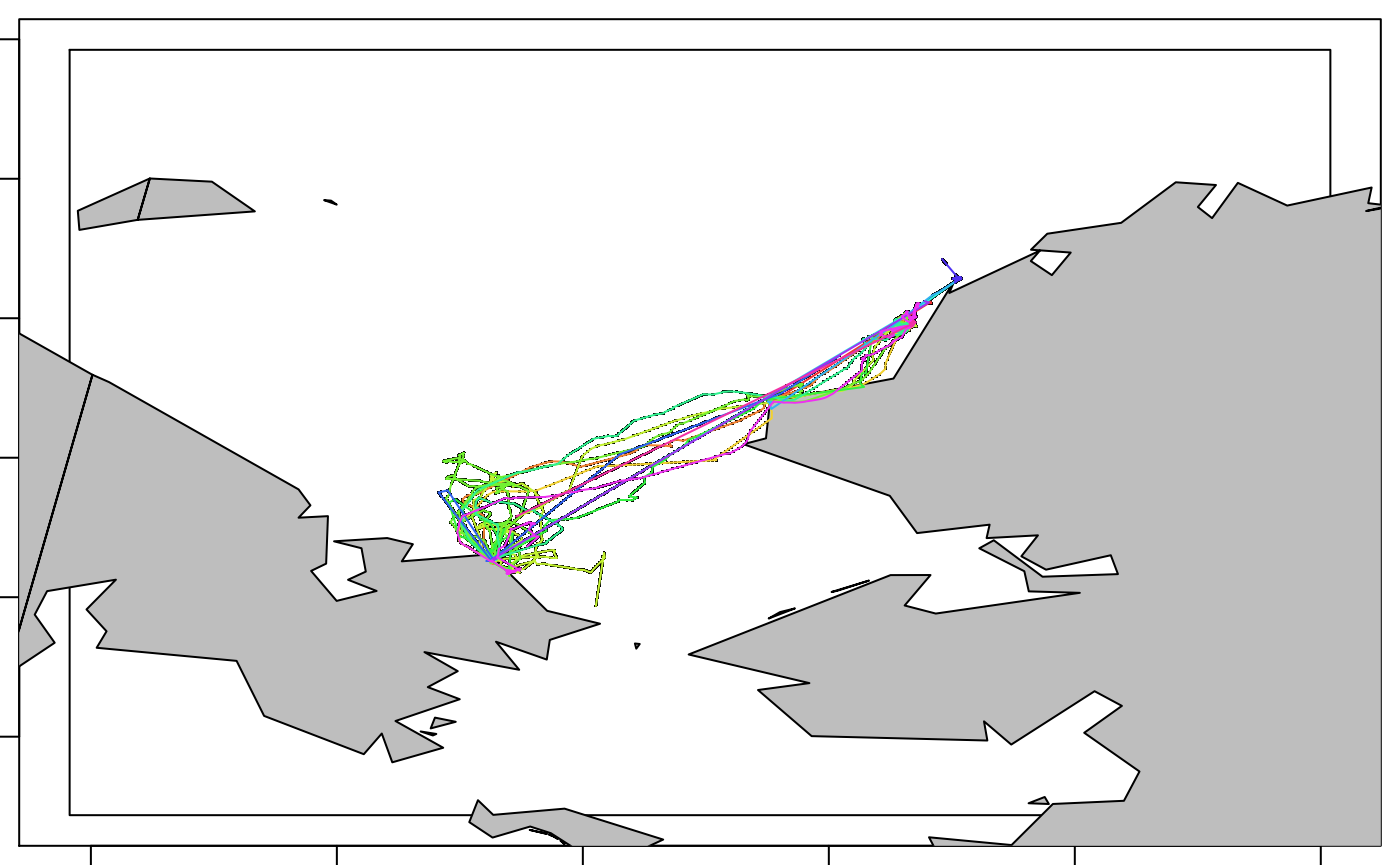
Data may be stored in longitude latitude or using a map projection, an in-built data set uses the Azimuthal Equidistant family near the anti-meridian in the Bering Strait.
raster::projection(walrus818)
## [1] "+proj=aeqd +lat_0=70 +lon_0=-170 +x_0=0 +y_0=0 +datum=WGS84 +units=m +no_defs"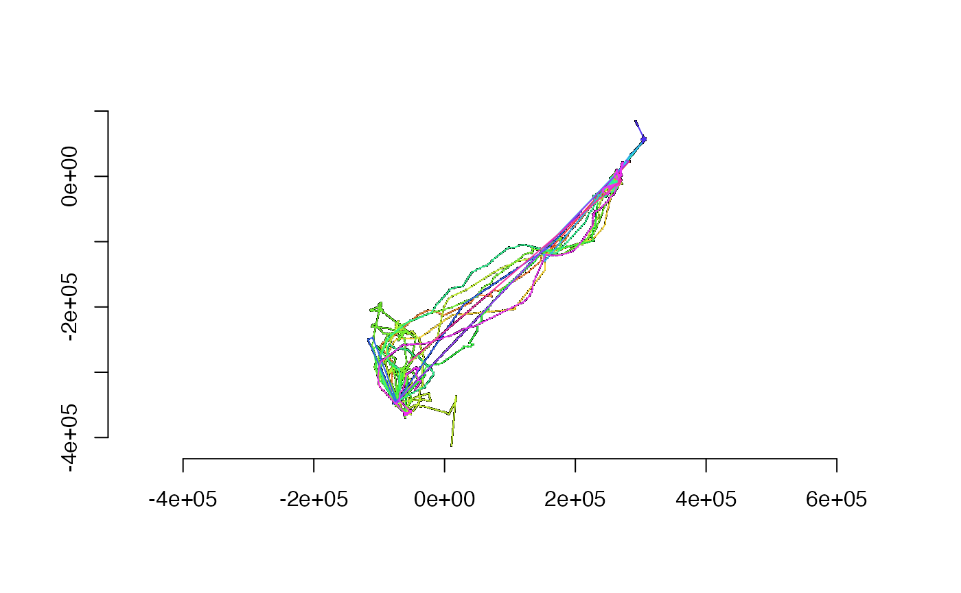
data("world_north", package= "trip")
p <- par(mar = rep(0.5, 4))
plot(raster::extent(walrus818) + 600000)
plot(walrus818, pch = ".", add = TRUE)
plot(world_north, add = TRUE, col = "grey")
lines(walrus818)
par(p)
Data conversions
There are various conversions from other tracking data types, the trip() function aims to be a helpful function like raster::raster(), simply understanding many formats.
It’s possible to export trips to Google Earth, for interacting with the time slider in continuous time. Use write_track_kml() to produce a ‘KML/KMZ’ file.
When converting to spatial forms we may choose multi-lines, points, or segments.
Conversion to points, in sp or spatstat.
## as points
as(walrus818, "SpatialPointsDataFrame")
## class       : SpatialPointsDataFrame
## features    : 10558
## extent      : -117277, 307789, -412557, 84896  (xmin, xmax, ymin, ymax)
## crs         : +proj=aeqd +lat_0=70 +lon_0=-170 +x_0=0 +y_0=0 +datum=WGS84 +units=m +no_defs
## variables   : 4
## names       : Deployment,     DataDT, Wet, Forage
## min values  :        353, 1252987200,   0,      0
## max values : 444, 1287601200, 1, 1as(walrus818, "ppp")
## Marked planar point pattern: 10558 points
## Mark variables: Deployment, DataDT, Wet, Forage
## window: rectangle = [-117277, 307789] x [-412557, 84896] units
Conversion to lines, in sp, sf, or adehabitatLT.
## as lines
as(walrus818, "SpatialLinesDataFrame")
## class       : SpatialLinesDataFrame
## features    : 14
## extent      : -117277, 307789, -412557, 84896  (xmin, xmax, ymin, ymax)
## crs         : +proj=aeqd +lat_0=70 +lon_0=-170 +x_0=0 +y_0=0 +datum=WGS84 +units=m +no_defs
## variables   : 4
## names       : tripID,  tripStart,    tripEnd, tripDur
## min values  :    353, 1252987200, 1254337200, 1195200
## max values : 444, 1283878800, 1287601200, 5695200class(as(walrus818, "sf"))
## Warning in sp::proj4string(from): CRS object has comment, which is lost in
## output
## [1] "sf" "data.frame"class(as(walrus818, "sf")$geom)
## Warning in sp::proj4string(from): CRS object has comment, which is lost in
## output
## [1] "sfc_LINESTRING" "sfc"as(walrus818, "ltraj")
## Loading required namespace: adehabitatLT## Registered S3 methods overwritten by 'adehabitatMA':
## method from
## print.SpatialPixelsDataFrame sp
## print.SpatialPixels sp##
## *********** List of class ltraj ***********
##
## Type of the traject: Type II (time recorded)
## * Time zone: GMT *
## Irregular traject. Variable time lag between two locs
##
## Characteristics of the bursts:
## id burst nb.reloc NAs date.begin date.end
## 1 353 353 160 0 2009-09-15 04:00:00 2009-09-30 19:00:00
## 2 354 354 813 0 2009-09-16 04:00:00 2009-10-20 00:00:00
## 3 355 355 1151 0 2009-09-16 04:00:00 2009-11-04 19:00:00
## 4 356 356 1534 0 2009-09-16 23:00:00 2009-11-21 21:00:00
## 5 357 357 1274 0 2009-09-16 23:00:00 2009-11-09 22:00:00
## 6 358 358 596 0 2009-09-16 23:00:00 2009-10-18 19:00:00
## 7 359 359 1053 0 2009-09-16 23:00:00 2009-10-30 19:00:00
## 8 361 361 556 0 2009-09-17 01:00:00 2009-11-06 04:00:00
## 9 362 362 301 0 2009-09-17 01:00:00 2009-10-03 17:00:00
## 10 366 366 405 0 2009-09-19 15:00:00 2009-10-12 20:00:00
## 11 367 367 1172 0 2009-09-17 01:00:00 2009-11-10 16:00:00
## 12 368 368 151 0 2009-09-19 02:00:00 2009-10-02 22:00:00
## 13 443 443 1035 0 2010-09-07 17:00:00 2010-10-20 19:00:00
## 14 444 444 357 0 2010-09-07 17:00:00 2010-09-28 05:00:00
##
##
## infolocs provided. The following variables are available:
## [1] "pkey"Conversions to segments, in sp, spatstat.
## as segments
explode(walrus818)
## class       : SpatialLinesDataFrame
## features    : 10544
## extent      : -117277, 307789, -412557, 84896  (xmin, xmax, ymin, ymax)
## crs         : +proj=aeqd +lat_0=70 +lon_0=-170 +x_0=0 +y_0=0 +datum=WGS84 +units=m +no_defs
## variables   : 4
## names       :  starttime,    endtime, timedur,  id
## min values  : 1252987200, 1252990800,    3600, 353
## max values : 1287597600, 1287601200, 2152800, 444as(walrus818, "psp")
## marked planar line segment pattern: 10544 line segments
## Mark variables:  origMarks, pattern
## window: rectangle = [-117277, 307789] x [-412557, 84896] units
Why not sf?
The trip package cops a bit of dismissive criticism because it’s based on sp which is somehow seen as hopelessly legacy. Trip uses sp in powerful ways, but the greatest power is
- no dependence on unnecessary libs (no GDAL, no GEOS)
- efficient storage of points
There’s some excitement about the new sf package, and some moves to write yet another trajectory formalism based on sf. I would never use it, sf is a non starter for track data. If these things change I would reconsider, but I don’t see that happening as sf is extremely brittle now, also these suggestions were made early and ignored.
- simple features (the standard) is not capable of storing tracking data
- sf splits up sets of points in a list
- sf brings GDAL and GEOS along with it with no opt-out.
Trip has a lot of problems, but these basic things are just no-go. It’s been said trip is only point-based, but the time-spent gridding, the speed filtering, and the conversion to line segments is all clearly line-based. I’m still looking for sensible collaboration for a better system in R, but to me it’s as simple as a grouped data frame with dplyr/ggplot2 semantics. Anything more requires a multi-table system and shoe-horning into the sf straitjacket is not going to work.
See vignette ‘trip-rationale’ for a longer version.
One-dimensional, are you crazy? Yes, the measurement process is one-dimensional and that is how we can arrange the primary data we collect. We collect location (x, y, z), time, and many other variables such as temperature, air pressure, happiness and colour, these are the geometry of our measurements, but the collection itself is very much a one-dimensional topology.↩︎