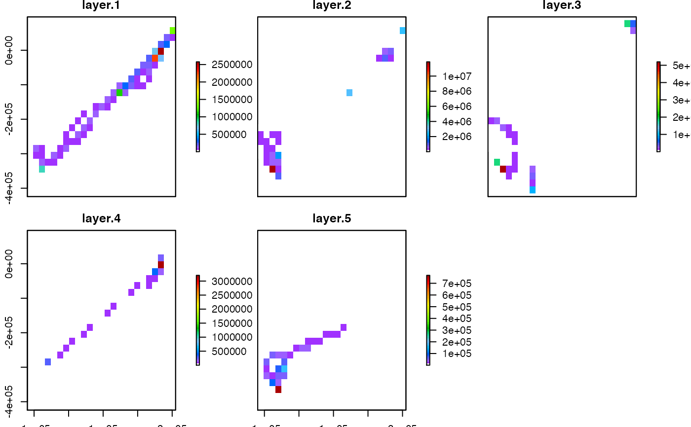
Split trip events into exact time-based boundaries.

Split trip events within a single object into exact time boundaries, adding interpolated coordinates as required.

# S3 method for trip
cut(x, breaks, ...)

Arguments

x	A trip object.
breaks	A character string such as the `breaks` argument for `cut.POSIXt`, or alternatively a vector of date-time boundaries. (If the latter these must encompass all the time range of the entire trip object.)
...	Unused arguments.

Value

A list of trip objects, named by the time boundary in which they lie.

Details

Motion between boundaries is assumed linear and extra coordinates are added at the cut points.

This function was completely rewritten in version 1.1-20.

Author

Michael D. Sumner and Sebastian Luque

Examples


if (FALSE) {
set.seed(66)
d <- data.frame(x=1:100, y=rnorm(100, 1, 10),
                tms= as.POSIXct(as.character(Sys.time()), tz = "GMT") + c(seq(10, 1000, length=50),
                seq(100, 1500, length=50)), id=gl(2, 50))
sp::coordinates(d) <- ~x+y
tr <- trip(d, c("tms", "id"))

cut(tr, "200 sec")

bound.dates <- seq(min(tr$tms) - 1, max(tr$tms) + 1, length=5)
trip.list <- cut(tr, bound.dates)
bb <- bbox(tr)
cn <- c(20, 8)
g <- sp::GridTopology(bb[, 1], apply(bb, 1, diff) / (cn - 1), cn)

tg <- tripGrid(tr, grid=g)
tg <- sp::as.image.SpatialGridDataFrame(tg)
tg$x <- tg$x - diff(tg$x[1:2]) / 2
tg$y <- tg$y - diff(tg$y[1:2]) / 2

op <- par(mfcol=c(4, 1))
for (i in 1:length(trip.list)) {
  plot(sp::coordinates(tr), pch=16, cex=0.7)
  title(names(trip.list)[i], cex.main=0.9)
  lines(trip.list[[i]])
  abline(h=tg$y, v=tg$x, col="grey")
  image(tripGrid(trip.list[[i]], grid=g), interpolate=FALSE,
  col=c("white", grey(seq(0.2, 0.7,  length=256))),add=TRUE)
  abline(h=tg$y, v=tg$x,  col="grey")
  lines(trip.list[[i]])
  points(trip.list[[i]], pch=16, cex=0.7)
}

par(op)
print("you may need to resize the window to see the grid data")

cn <- c(200, 80)
g <- sp::GridTopology(bb[, 1], apply(bb, 1, diff) / (cn - 1), cn)

tg <- tripGrid(tr, grid=g)
tg <- sp::as.image.SpatialGridDataFrame(tg)
tg$x <- tg$x - diff(tg$x[1:2]) / 2
tg$y <- tg$y - diff(tg$y[1:2]) / 2

op <- par(mfcol=c(4, 1))
for (i in 1:length(trip.list)) {
  plot(sp::coordinates(tr), pch=16, cex=0.7)
  title(names(trip.list)[i], cex.main=0.9)
  image(tripGrid(trip.list[[i]], grid=g, method="density", sigma=1),
        interpolate=FALSE,
        col=c("white", grey(seq(0.2, 0.7, length=256))),
        add=TRUE)
  lines(trip.list[[i]])
  points(trip.list[[i]], pch=16, cex=0.7)
}

par(op)
print("you may need to resize the window to see the grid data")

}

data("walrus818", package = "trip")
library(lubridate)
#> 
#> Attaching package: ‘lubridate’
#> The following objects are masked from ‘package:base’:
#> 
#>     date, intersect, setdiff, union
walrus_list <- cut(walrus818, seq(floor_date(min(walrus818$DataDT), "month"), 
ceiling_date(max(walrus818$DataDT), "month"), by = "1 month"))
g <- rasterize(walrus818) * NA_real_
stk <- raster::stack(lapply(walrus_list, rasterize, grid = g))
st <- raster::aggregate(stk, fact = 4, fun = sum, na.rm = TRUE)
st[!st > 0] <- NA_real_

plot(st, col = oc.colors(52))